🇪🇺 🇺🇸 Euro Macromechanica (EMM) Backtest — Overview & Methodology
Euro Macromechanica — Macro-structural Mechanics of EUR/USD
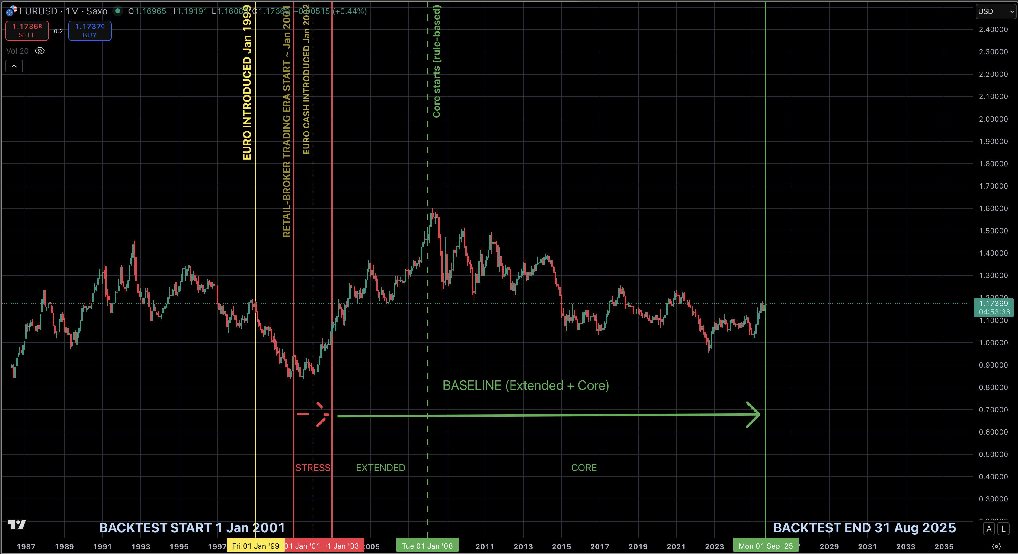
Backtest Period Map (EUR/USD, 2001–2025-08)
Note: “quant” is short for quantitative.
A full guide for verifying the transparency of the processes and the input/output files used in the backtest is provided in AUDIT.md; the link is also repeated at the end of this document.
The project results provide robust empirical evidence of invariant quantitative factors (signals of market inefficiency) in EUR/USD price dynamics over the entire historical backtest period. Consistent outcomes over nearly the entire history of the euro as the EU’s single currency (since the introduction of cash in January 2002), including the major systemic crises of the past two decades, corroborate this.
This project should not be regarded as a “full-fledged institutional-level micro-backtest”. Rather, it serves as an indirect demonstration of the sustainable effectiveness of a single research model, EMM, based on the results of the base core on M5 under a conservative execution framework. The base core represents the minimal necessary sample of trades for the EMM research, derived from a limited set of quantitative factors. Its purpose is to illustrate performance potential, rather than to provide high-precision metrics, which is inherently unattainable at a non-institutional level, particularly given the OTC-specific context.
The backtest project includes, in particular:
- coverage of nearly the entire history of the euro as the EU’s single currency, including all major systemic crises of the past two decades;
- only one intraday signal logic on the M5 timeframe;
- a fully unchanged logic (no retraining) across the entire backtest horizon;
- a transparently verifiable pipeline of input and output data (deterministic execution, a cryptographic hash chain, and unedited, single-take live backtest recordings) without disclosing the strategy logic;
- a technically thorough engine implementation, with emphasis on objective treatment of all relevant factors and maximal accounting of all plausible trading costs under non-institutional infrastructure and constrained resources;
- transparent metric computation based on non-public trade files and equity series (cryptographically anchored in the consolidated result manifests generated by the backtest engine), including an open calculator script and the calculation methodology;
- consistentl results over the entire backtest horizon on a single asset — EUR/USD.
- GBPUSD cross-asset test over the main data-quality period 2008–2025-08, including both pre-Brexit and post-Brexit (2016) periods.
The backtest was conducted in UTC (UTC+0).
Table of Contents
- Input Data for the M5 EMM Backtest
- Public Logic of the M5 EMM Engine
- Implemented M5 EMM Strategy Logic
- M5 EMM Cost Model (EUR/USD) Methodology
- Rationale for a Look-Ahead-Free Implementation of the Mathematical Computation of Objective (TP) and Guard (SL) Levels on Fully Formed 5-Minute Bars in the M5 EMM Engine
- Rationale for Choosing HistData Minute Data for the M5 EMM Backtest
- Results: Data Quality Policy v1.0 Periods, Profiles, Risk Modes, Capitalization Modes, and Determinism
- Evidence of Strategy Existence and Invariance
- Metrics
- Brief Results Overview
- Conclusions
- Limitations and scope of applicability
- Links
- Contact
- Licenses and Attributions
- Disclaimer — Not Investment Advice
Input Data for the M5 EMM Backtest
Source Minute Data, Data Quality Policy, and the Decision to Split Backtest Periods
The euro was introduced as the EU’s single currency in non-cash form in January 1999; retail access to EUR/USD trading emerged around 2001. Cash euros were introduced in January 2002.
The primary objective is to run the backtest over the longest feasible horizon, ideally starting from the point when retail access via FX brokers became available.
Special thanks to HistData for free access to minute data (and tick samples) for currency pairs with broad historical coverage—one of the few free sources comparable in scope.
A decision was made to conduct the backtest on minute data from HistData rather than on ticks. The rationale for choosing minute data and the HistData source (versus alternatives such as Dukascopy) is described in the section “Rationale for choosing HistData minute data for the M5 EMM backtest.”
Unfortunately, the quality of the minute data did not allow for a robust test of 2001–2002: the number of 5–15 minute gaps was exceptionally high, which is critical for M5 logic (all quant factors are implemented on the M5 timeframe, and a large number of gaps in that range materially distorts the computation of the required levels). Therefore, 2001–2002 are used as a stress period to illustrate strategy behavior under degraded data quality. Accordingly, metrics are computed only for the baseline periods.
Data quality for 2003–2007 is also below the core period, so this span is labeled Extended Baseline to keep it separate from the higher-quality core period — Core Baseline (2008–2025-08). To illustrate results over the longest horizon, a composite track is also provided in a compounding mode (balance carries forward year to year: Ending Balance → next year’s Initial Balance) on mixed-quality data — Composite Baseline (2003–2025-08 = extended + core).
Gaps exceeding 15 minutes are also material, but their impact is lower relative to 5–15 minute intervals. Consequently, the 5–15 minute range is adopted as the key band for classification. In an ideal setting there would be no gaps at all; the work proceeds with the data that were available at the time.
Backtest periods:
- Stress period: 2001–2002 (illustrative runs on degraded data quality).
- Extended Baseline: 2003–2007 (5 years).
- Core Baseline: 2008–2025-08 (17 years 8 months).
- Composite Baseline: 2003–2025-08 (22 years 8 months).
Metrics are published only for the baseline periods. (Extended metrics are provided only for the Core Baseline.)
According to HistData, the raw minute data are timestamped in fixed EST (UTC−5) (see the F.A.Q.: http://www.histdata.com/f-a-q/). For the backtest, they are normalized to UTC (UTC+0).
Minute-data normalization includes only:
- assigning column names:
datetime,open,high,low,close,volume; - converting timestamps to UTC (UTC+0) and sorting.
The minute data values were neither modified nor removed.
- Normalized minute data — data-hub/source_data/prepared
- Minute-data normalization script — data-preparation-toolkit/minute_data_normalizer
- Gap-report analysis script for minute data — data-preparation-toolkit/minute_data_analyzer
All original minute-data files and text reports on minute-data quality were obtained from HistData. The gap analysis is fully reproducible with any tools. A simple visual inspection of the frequency of 5–15-minute gaps confirms the appropriateness of the chosen Data Quality Policy and addresses skeptical concerns (including assertions about possible OTS “timeline anchoring,” etc.). The raw minute data sourced from HistData are likewise fully reproducible. If HistData requests data removal, the raw minute files used in the backtest will be made available for verification upon request.
Economic Calendars
The calendars were compiled manually (in parts) with the assistance of ChatGPT’s advanced modes: official sources throttle bulk HTTP requests, and there are no free consolidated calendars covering such a long period. The engine required a narrow set of countries and only key macro releases, specifically filtered by the author, which are typically published within fixed time windows. Accordingly, the risk of potential timing inaccuracies in the collected releases is low.
All events are sourced from official websites: national central banks, national statistical agencies, etc.
In the implemented logic, the calendar serves as an entry filter, not a signal source: the strategy avoids opening positions during release windows. If a release time is incorrect, a trade will typically be closed via stop-loss rather than generate “false” profit. Consequently, even in the unlikely presence of timing errors, the results are generally more likely to be understated than overstated.
List of high-importance events and countries specifically filtered and compiled for the M5 EMM engine.
United States:
- Scheduled FOMC events: press conferences, statements, and rate decisions
- Fed Chair speeches at the Jackson Hole Economic Symposium
- Semiannual testimony by the Federal Reserve Chair before the U.S. Congress on the Monetary Policy Report (Humphrey–Hawkins)
- Employment Situation (Nonfarm Payrolls, NFP)
- GDP (BEA: advance/second/third)
- Retail Sales (Advance, Census)
- ISM Manufacturing PMI
- ISM Services PMI (officially “ISM Services PMI”; formerly Non-Manufacturing)
- PCE Price Index
- CPI
- PPI
Euro Area:
- Scheduled ECB press conferences and rate decisions
Reasons for excluding flash HICP, Unemployment Rate, etc. for the Euro Area
- First, these releases generally do not drive ≥60-pip EUR/USD moves within the 10–15-minute window after publication. They are therefore immaterial to the implemented logic; rare, episodic spikes on flash HICP do not change the overall picture.
- Second, the engine logic is designed to capture impulses on the order of ~40 pips and larger over 5–10 minutes.
Details of the implemented logic in the M5 EMM backtest are provided in the section Implemented M5 EMM Strategy Logic.
Unscheduled high-importance events (e.g., ad-hoc FOMC decisions/statements, inter-meeting actions) were recorded separately as a precaution, but they were not included in the scheduled calendars and were not used in the backtest, as they are not scheduled publications.
Economic calendars are available at data-hub/economic_calendars/.
The directory data-hub/economic_calendars/raw/ contains the collected calendars with events in each source’s local release time, split into parts for greater transparency. The directory data-hub/economic_calendars/prepared/ contains the normalized calendars — converted to UTC+0 — that were used as input files in the backtest.
The calendars do not include actual release values—only metadata such as time, title, importance, country/region, etc.
Calendar normalization consists only of converting publication times to UTC+0 and sorting the records. The UTC+0 conversion uses the IANA time-zone database, ensuring correct handling of local rules and Daylight Saving Time (DST) transitions. There are no DST-related inconsistencies: the key macro releases listed above are not published during clock-change hours.
Calendar normalization script — data-preparation-toolkit/economic_calendar_normalizer
All calendar data used in the backtest are fully transparent and reproducible.
Public M5 EMM Engine Logic
Input Normalization and Determinism
The engine ingests one-minute market data and calendar events timestamped in UTC (ISO-8601). Before simulation, all input series are brought to a single, reproducible form so that the outcome depends only on the data themselves, not on row order, duplicates, or source artifacts. One-minute records are ordered by time; if multiple rows share the same timestamp, the last one is retained and the preceding ones are treated as superseded; malformed or incomplete price values are discarded. No synthetic fills or interpolations are applied—only the actual content of the data is used in calculations.
Minutes are then mapped unambiguously to five-minute windows by interval membership: empty windows are dropped; partially filled windows are preserved without fills/interpolations. Normalization does not create missing minutes, so real gaps are preserved and handled by the gap logic.
Calendar data (hourly events and trading schedules) are normalized to a common format and de-duplicated; their application is described in the section Implemented M5 EMM Strategy Logic.
Normalization and aggregation procedures are deterministic: given identical inputs, repeated runs yield identical results regardless of the original row order, the presence of duplicates, or heterogeneity of the export. At the end of the period, any remaining positions are closed at the last available one-minute price, which fixes the terminal state unambiguously.
Determinism of results.
Simulation outcomes are deterministic: with identical inputs, repeated runs reproduce the same set of trades, timestamps, and prices. This is achieved through stable sorting and de-duplication, a fixed grid and rules for mapping minutes to windows, an unambiguous choice of the “earliest” minute where applicable, a single global epsilon, a fixed SL-over-TP priority in conflict cases, strict quant-logic rules, and the absence of randomness. Partially filled bars are preserved without interpolation; real gaps are not filled and are handled by the gap logic. For exact reproducibility, the M5 EMM engine’s dependency versions are pinned.
Determinism of output files.
Simulation artifacts are produced deterministically: with unchanged inputs, parameters, and dependency versions, each rerun produces the same set of files with identical content. This is ensured by a uniform time base and fixed M5 grid, prior normalization of one-minute records (stable sorting, de-duplication without interpolation), a predictable, staged simulation pipeline (a two-pass scheme that forms trades and equity snapshots, aligns equity to entry times, and a final pass without random components), and stable serialization rules (constant delimiter, fixed numeric precision, a single timestamp format, and time-ordered rows). The composition and naming of outputs remain constant via templates with deterministic year resolution; the SVG visualization is generated from the already-deterministic equity series and is therefore reproducible as well. For external verification of immutability, an artifacts_YYYY.sha256 file is produced listing the SHA-256 checksums of all input and output artifacts; its lines are sorted so the checksum file itself is byte-stable. With identical inputs/parameters and pinned library versions, the contents of trades_YYYY.csv*, balance_YYYY.csv* (equity series), summary_YYYY.csv*, balance_YYYY.svg, and artifacts_YYYY.sha256 are byte-for-byte identical across runs.
Aggregating Minutes into M5 Bars
Minute quotes are mapped onto a fixed five-minute grid: a window starts at time t and covers the half-open interval [t, t + 5 minutes), with each minute belonging to exactly one window. One M5 bar is produced per window: Open comes from the earliest valid minute in the window, High/Low are the maximum/minimum across the minutes in the window, and Close comes from the latest valid minute in the window. If a window contains no valid minutes, no bar is created; if it contains fewer than five minutes, the bar is treated as partially filled and is preserved without padding or interpolation. The bar’s timestamp is the window start time (t).
Aggregation is performed after minute-level normalization and deduplication.
The procedure is deterministic: the order of input rows and duplicate occurrences of the same minute timestamp do not affect the result (when timestamps collide, the last record is used). Partially filled bars are retained; their eligibility for entry searches is governed by data-quality rules and the trading schedule. When a gap is detected, only new entries are temporarily blocked, while management of already open positions continues.
Order Execution Logic
- On each M5 bar, a deterministic set of auxiliary levels in the trade direction is computed from the current M5 bar and the history of prior M5 bars: Trigger (entry), Guard (SL) (stop), and Objective (TP) (profit-taking target).
- Levels are not recomputed within the 5-minute window; a new set appears only when the window rolls to the next M5 bar.
- At most one trade per computed Trigger level.
- Monitoring operates on the M5 grid; the actual fill is searched on M1 within the current M5 bar.
- If multiple M1 candles touch the Trigger within an M5 bar, the earliest touching minute executes. Guard (SL) and Objective (TP) follow the same earliest-touch rule.
- Guard (SL) is fixed at entry (the minute the Trigger executes) and is calculated relative to the current M5 bar. Objective (TP) is dynamic and is recomputed on each subsequent M5 bar after entry.
- If the Objective (TP) is reached within the current M5 bar, the trade closes at the level computed for the current bar; if the first minute of the next M5 bar has begun and the Objective is then reached, the close occurs at the next bar’s level.
- A computed Guard (SL) is required to open a trade. Requiring a pre-computed Objective (TP) at entry is deliberately omitted for conservatism: if it is missing at entry, the Objective is computed on the next M5 bar and thereafter, until a stop occurs.
- If two Trigger levels are reached in the same minute within an M5 bar, trades are opened from both levels; risk is taken as the configured per-trade risk from the balance at entry (e.g., with a $100,000 balance and 1% risk per trade, each trade risks 1%—the risk is not split).
- When TP and SL are both touched on M1, Guard (SL) always has priority.
- If two Trigger levels are reached in different minutes within the same M5 bar, trades are opened from each Trigger accordingly.
The implemented logic uses market orders. For details of the market-order cost model, see
M5 EMM Cost Model (EUR/USD) Methodology.
For the rationale behind computing Objective (TP) and Guard (SL) from fully formed M5 bars (rather than incrementally within the current bar; i.e., look-ahead considerations), see
Rationale for a Look-Ahead-Free Implementation of the Mathematical Computation of Objective (TP) and Guard (SL) Levels on Fully Formed 5-Minute Bars in the M5 EMM Engine
Order Execution Logic in the Presence of Gaps
After entry, the position is tracked on M1 within the current M5 bar. If a gap occurs (no minutes inside one or more M5 bars), the close check resumes on the first available minute after the gap. The close is executed at the computed level, not at the opening price of the first minute after the gap.
- Guard (SL) is fixed at entry (from the M5 bar where the Trigger fired) and does not change. After a gap, as soon as the first available M1 minute reaches Guard (SL), the trade closes at the Guard (SL) level (the level is constant). Thus, the stop does not gain from the gap and is not “improved.”
- Objective (TP) is dynamic:
- if the Objective (TP) is reached within the same M5 bar, closing occurs at that bar’s Objective (TP);
- if the first available minute is already in the next M5 bar and the target would have been reached during the gap, the close occurs at the next bar’s Objective (TP) (i.e., the freshly recomputed level on the new bar), not at the post-gap opening price.
- There is no windfall from gaps. Even if the market “jumps” far beyond the target, the close is executed at the computed Objective (TP) of the relevant M5 bar (current/next), not at a potentially better post-gap opening price. Likewise, loss is fixed at the predetermined Guard (SL).
- Potential deviation due to a 5-minute gap: because Objective (TP) is recomputed on each new M5 bar, its value after a gap may differ slightly from the hypothetical level without a gap—either upward or downward. Accordingly, this does not confer an unintended advantage to the strategy.
- Conflict on the first minute after a gap (if both Guard (SL) and Objective (TP) would be touched): Guard (SL) always has priority.
Gap-Detection Logic
The detector evaluates each M5 bar by comparing:
-
Time gap between
• the last minute before the start of the current timeframe (TF) window, and
• the first minute inside the current TF window.
If this pause is strictly greater than the configured threshold (in minutes), a gap is recorded. -
Price gap between
• the close of the last minute of the previous window, and
• the open of the first minute of the current window.
If the absolute difference is ≥ the configured threshold (in pips), a gap is recorded. (Threshold set to 25 pips.)
The checks apply only if both the “previous minute” and the “first minute of the current window” are available. If either is missing, no gap is detected on that bar.
If the pause before the start of the current window exceeds a separate “long” reopen threshold of 1440 minutes, then—even if the above conditions are met—the gap does not trigger a lockout (it is treated as a normal reopen after a long break such as weekends/holidays). If at least one type of gap (time or price) is detected and this is not a reopen, the lockout window starts at the first minute of the current TF window where the gap was detected. The lockout duration is configured in minutes. (Set to 30 minutes.)
While the current M5 bar falls within the lockout window, only new entries are disallowed. Management and exits of already open positions proceed as usual. If an M5 bar has no minutes at all, the bar is skipped entirely, and management/exits are not evaluated on it. When the current TF time reaches (or is past) the end of the lockout, the lock is removed and normal processing resumes.
Gap checking is performed inside the entry-eligibility branch (after external quant factors) and before testing Trigger touches. A lockout window is set if the bar is eligible for entries and a gap is detected, regardless of whether any Trigger touch occurs. If the bar is not eligible or this is a reopen, no lockout window is set—by design, for conservatism, to avoid additional filtering where entries are not possible anyway.
Implementation Notes
- Empty M5 bars. If the current M5 bar contains no M1 minutes, the bar is skipped entirely: no gap detection, no new-entry checks, and no position management/exits are performed (there is nothing to evaluate). Management resumes at the first available minute of the next bar.
- The time threshold is compared as
>(strictly greater), the price threshold as≥. - The lockout always starts at the first minute of the current window; if both checks (time and price) trigger simultaneously, the result is the same.
- The lockout does not accumulate and is not auto-extended; a new lockout may start on the next bar if another gap is detected.
- “Extension” of the lockout.
- If the next eligible bar also contains a gap, the engine starts a new lockout window from that bar’s start—effectively resetting the timer. This may look like an extension, but it is not a sum of intervals; it is a new window that overwrites the previous start/end by time.
- If a bar is empty (no M1 minutes), it is skipped entirely: no entry checks, no gap detection, and no extension/restart of the lockout window occur on it.
- If the reopen threshold is hit, the lockout is not enabled, even if regular gap thresholds are exceeded.
The gap detector evaluates only the M5 window boundary—the interval between the last M1 before the window and the first M1 inside the window. Missing minutes inside the window are not treated as a gap, and no lockout window is started because of them.
Two data-quality rules apply:
- Thin bar. If a window contains too few minutes, the bar may be ineligible for entry searches by a minimum coverage threshold (set to 3 minutes). This is not a gap and does not start a lockout.
- Empty bar. If an M5 bar has no minutes at all, the bar is skipped in full; management/exits are not evaluated (there are no minutes to check).
Result: a lockout is triggered only by a boundary gap (time or price). Gaps inside an M5 window are neither detected nor penalized.
Due to the gap-protection logic, some potential trades may be skipped; however, given the 2008–2025-08 data quality, such cases are rare. Detecting gaps specifically at M5 window boundaries further filters discontinuities to increase result objectivity. The rationale for boundary-based lockouts is that Trigger / Guard / Objective levels are fixed at the close of each M5 bar (from bar data) and are not recalculated inside the bar. A new level set appears only at a window change, hence the natural place to check for gaps is the boundary (last M1 before the window vs. first M1 inside). Gaps inside an M5 bar do not start a lockout: levels are static within the bar, so the bar-eligibility filter suffices without extra blocking. Introducing lockouts for intra-bar gaps would be overly strict; for such gaps, the bar’s entry-eligibility filter is applied without starting a lockout.
Gap detection is applied exclusively within the entry-eligibility branch (and before testing Trigger touches); outside this context it is not activated. This design avoids over-filtering rare minute-data artifacts and prevents unnecessary noise in the backtest. Empirically, the approach is supported by the stability of long-horizon backtest results under the data-quality period classification.
Cost Accounting, Trade Size Calculation, and Rounding
The engine is configured with fixed cost parameters for a single annual run (within the selected profile/mode and calendar year). Costs comprise commission, spread, and slippage. All three components are applied to every trade; the published results already include their impact on PnL.
Point vs pip. For five-decimal quotes, 1 pip = 10 points. All thresholds/costs are specified in pips and converted to price.
- Commission. Specified as a round-turn rate per 1 standard lot (100,000 EUR) and applied proportionally to the actual position size. It is not included in per-trade risk sizing (size/lot sizing) — it is treated as a separate trading cost booked on top of the trade result.
- Spread and slippage. Specified as round-turn amounts (in pips) for the chosen profile/year and split evenly (50/50) between the two sides of the trade: half at entry, half at exit (e.g., spread RT = 0.8 pips ⇒ 0.4 / 0.4 pips). Spread and slippage are modeled via effective execution prices: entry/exit levels (Trigger/Objective/Guard) are shifted adversely. These costs are also included in position-size calculation at the target risk (lot sizing and expected stop loss are computed using the already adjusted prices), hence they directly affect final PnL.
- Fixed for the period. Cost parameters are set at launch and do not change within an annual run. Each profile/mode and calendar year uses its own values from the cost-model table aligned with the implemented M5 EMM cost-model logic —
docs/cost_model/m5_emm_cost_model_v1.0.csv.
For methodology details, see the section
M5 EMM Cost Model (EUR/USD) Methodology.
Bottom line: commission is accounted for separately from risk, while spread/slippage are included in risk and position-size calculations; all costs are applied to every trade, so run results and summary metrics already reflect their impact.
Per-trade position sizing. The position size for each trade is a fixed fraction of the current balance at entry (the risk fraction is set for the entire annual run). Risk is taken from the actual balance right before opening the trade, not from a pre-fixed notional.
If two Trigger levels are hit within the same minute of an M5 bar, trades are opened from both levels; the default per-trade risk is taken for each trade from the balance at entry (e.g., with a $100,000 balance and 1% risk per trade, both trades open at 1% risk each — the risk is not split between them).
Risk-based lot rounding. First, a “raw” position size is computed so that the potential loss at the stop equals the target risk; the stop distance is taken including spread/slippage. The size is then always rounded down to the nearest permissible increment, so the realized stop-risk does not exceed the target. Exceedance is only possible in edge cases:
- the computed lot is below the technical minimum and the minimum tradable size is used;
- multiple trades are opened in the same minute without splitting the overall per-minute risk cap between them;
- commission is charged on top of the trade result and increases the realized loss, since it is not included in the risk base.
Spread and slippage are explicit inputs and are included at the lot-sizing stage: the entry-to-SL distance is measured with these costs already applied.
Epsilon (ε)
The model uses a single comparison tolerance ε equal to one minimum tick increment of the instrument. For EURUSD (5-digit quotes): ε = 0.00001 (1 point = 0.1 pip).
Scope.
ε is used only for the binary check of whether a computed level is “touched” by the minute bar’s extremum (High/Low) within an M5 window. ε does not affect the computation of the levels themselves.
Order relative to costs.
First, the “touch / no-touch” event is determined with ε; then the execution price is formed with the configured costs (spread / slippage / commission). ε does not change the magnitude of the costs.
Exceptions (where ε is not applied).
Gap detection and bar-eligibility checks are evaluated strictly by the specified inequalities (> / ≥) without ε.
Rationale.
A value of 0.1 pip is minimally sufficient to offset boundary discretization and rounding effects on M1. It does not “widen” levels into zones and does not create a methodological advantage; any shifts are smaller than the tick size and far below transactional noise (spread / slippage / commission).
Determinism.
A fixed ε ensures reproducible results given identical inputs.
Related execution rules.
In intra-minute conflicts, Guard (SL) has priority over Objective (TP) when both are reached simultaneously.
Note (OTC specifics).
Minute OHLC series from different providers (e.g., HistData vs. Dukascopy) can differ slightly due to time zone, price type, and aggregation. Formalizing ε standardizes the “touch” criterion and reduces the impact of such differences.
Implemented M5 EMM Strategy Logic
This M5 EMM implementation covers the core—approximately 10–15% of the full strategy — representing a minimally sufficient set of trades to demonstrate effectiveness. In this design, all operations—trading decisions, computations, and feature handling — are performed exclusively on the 5-minute timeframe. The M5 module is not complete: owing to the approach’s complexity and resource constraints, the full suite of quantitative factors has not been implemented even within a single M5 model. Moreover, the current version does not include the principal logic for trading in post-release windows for major macroeconomic data, which is one of the key drivers of performance. The full EMM strategy is a composition of signals across the M1, M5, M15, M30, and H1 timeframes, incorporating macro-structural dynamics of the U.S. Dollar Index under a proprietary methodology; nonetheless, this M5 core is sufficient to demonstrate effectiveness.
Time Filters of the Implemented M5 EMM Logic
The strategy trades macro-structural patterns on M5 bars and opens positions only during calm intervals of the trading day. This is not “Asia-only”: “calm” refers to windows outside the volatile top-of-hour intervals in the London–NY sessions, the rollover period, and scheduled data-release windows; filters are also applied within active London–NY segments. All prohibitions are specified as fixed UTC windows and do not depend on DST (the HistData source’s fixed EST baseline is accounted for; see the FAQ: http://www.histdata.com/f-a-q/).
Within the EMM logic, 10-minute blocks are implemented as a filter for top-of-hour volatility in the active London–NY segments, where spreads/slippage statistically increase. Additional fixed filters prohibit or tighten entries at specific times based on EMM logic. The rollover and the CME Globex maintenance window are covered by a fixed block that spans both summer and winter.
FX rollovers (UTC):
- Summer (EDT, UTC−4): 21:00 UTC
- Winter (EST, UTC−5): 22:00 UTC
CME Globex daily maintenance break (UTC):
- Summer (CDT, UTC−5): 21:00–22:00 UTC
- Winter (CST, UTC−6): 22:00–23:00 UTC
A full no-trade window is enforced from 19:00 to 00:10 UTC, which covers the FX rollovers and the CME Globex break regardless of DST. Accordingly, by the time these windows begin there are no open positions, and no exits are executed during them. This is corroborated by trade metrics on average trade duration.
Calendar Filters of the Implemented M5 EMM Logic
Economic calendars are compiled only for pre-defined Euro Area and U.S. scheduled releases classified as high-importance. All timestamps are provided in UTC and are DST-agnostic.
-
Event hour (technical). Any calendar timestamp is mapped to its technical event hour, defined as the full hour starting at the beginning of that hour.
Example: a release at 15:30 is treated as the event hour 15:00–15:59. Tightening applies to the entire hour, not just from the release minute. -
Pre-window — full prohibition. The pre-window is 60 minutes before the release time. However, any portion that overlaps the event hour is governed by the event-hour rules (tightening rather than a full ban).
Effective pre-window: from (release time − 60 minutes) to the start of the technical event hour.
Example: for a 15:30 release, the raw window is 14:30–15:29:59, but 15:00–15:29:59 belongs to the event hour; therefore, the full prohibition effectively applies 14:30–14:59:59. -
Event hour — tightening (not a full ban). Throughout the technical event hour, trade entries are allowed only if a strict condition is met; in simplified form: price impulse ≥ 300 pips over 5–15 minutes. This threshold is a conservative upper bound; for EUR/USD such moves are rare. In such episodes, entries are more likely to occur 15–30 minutes or more after the release, when transaction costs (spread/slippage) typically normalize. Accordingly, even if such rare trades do occur, the specified cost model remains objective and does not bias results across the entire backtest horizon.
-
After the event hour. Beginning with the next hour mark (in the example, from 16:00), calendar constraints are lifted.
All filters, their values, and all quant logic are strictly fixed and uniform (no changes and no re-optimization) across the entire backtest horizon (profiles, risk modes, capitalization modes, etc.).
M5 EMM Cost Model (EUR/USD) Methodology
All components of the cost model—commission, spread, and slippage—are applied to every trade. Spread and slippage are incorporated into the orders’ effective execution price.
See Cost Accounting, Trade Size Calculation, and Rounding.
Commission Profiles
- Institutional — primary track: average institutional commission $5.5 per round-turn per 1 standard lot (100,000 EUR); equivalent ≈ 0.55 pips RT on EURUSD (≈ $2.75 per side) — benchmark for institutional conditions.
- Retail Rebate — average retail commission after cashback $5 per round-turn per 1 standard lot (100,000 EUR); equivalent ≈ 0.5 pips RT on EURUSD (≈ $2.5 per side) — rebate-account conditions.
- Retail Standard — illustrative retail commission: $7 per round-turn per 1 standard lot (100,000 EUR); equivalent ≈ 0.7 pips RT on EURUSD (≈ $3.5 per side).
Institutional
All institutional modes apply a fixed commission of $5.5 per round-turn per 1 standard lot (100,000 EUR) as a separate expense line, regardless of flow type (ECN/PoP raw-spread, single-dealer, “zero-commission,” etc.).
Equivalents: ≈ 0.55 pips RT (≈ $2.75 per side; $55 per $1M RT).
Spread and slippage are handled separately per the EUR/USD execution model from m5_emm_cost_model_v1.0.csv and do not include the commission. The total transactional cost equals (spread + slippage) plus the $5.5 RT/lot commission.
Rationale
- Normalizes metrics across liquidity providers and pricing models (line-item commission vs all-in spread).
- Improves auditability: the commission is an explicit parameter and can be varied in sensitivity checks without changing spread/slippage.
Market levels (reference)
A fixed value of $5.5 RT/lot is used in calculations; the table below is for comparison with market practice.
| Flow / Venue | Charging method | Typical level (RT/lot) | Pips RT (equiv.) | $ per $1M RT | Notes |
|---|---|---|---|---|---|
| Top-tier ECN / PoP (raw-spread) | Line-item commission | $4–6 | 0.40–0.60 | $40–60 | Benchmark for mid/large participants; $5.5 sits near mid. |
| Prime-broker direct, high volume | Line-item commission | $2–4 | 0.20–0.40 | $20–40 | Requires high volumes and tighter tiers. |
| Smaller PoP / low frequency | Line-item commission | $6–7 | 0.60–0.70 | $60–70 | Lower volume discounts; less regular trading. |
| Single-dealer (all-in) | Cost embedded in spread | — | +~0.3–0.7 pips | — | In the model, commission is separate (fixed $5.5). |
| “Zero-commission” ECN | $0/lot, wider spread | — | ~0.5–0.8 pips | — | All-in equivalent; commission entered separately. |
Conversions
- 1 lot = $10 per 1 pip ⇒ $X RT/lot = X/10 pips RT.
- $ per $1M RT = 10 × ($ per lot RT) = 100 × (pips RT).
Sensitivity (indicative)
-
Notional Volume (EUR): 5M (50 lots; $/pip = $500)
→ Base: $275 RT/trade (= 0.55 pips × $500)
→ Δ±$1 RT/lot ⇒ ±$50/trade (≈ ±0.10 pips RT) -
Notional Volume (EUR): 10M (100 lots; $/pip = $1,000)
→ Base: $550 RT/trade (= 0.55 pips × $1,000)
→ Δ±$1 RT/lot ⇒ ±$100/trade (≈ ±0.10 pips RT) -
Notional Volume (EUR): 15M (150 lots; $/pip = $1,500)
→ Base: $825 RT/trade (= 0.55 pips × $1,500)
→ Δ±$1 RT/lot ⇒ ±$150/trade (≈ ±0.10 pips RT) -
Notional Volume (EUR): 30M (300 lots; $/pip = $3,000)
→ Base: $1,650 RT/trade (= 0.55 pips × $3,000)
→ Δ±$1 RT/lot ⇒ ±$300/trade (≈ ±0.10 pips RT)
Formulas
- Commission per trade (RT, $):
Cost_RT_$ = Commission_RT_per_lot_$ × (Notional_USD / 100,000) - Commission in pips RT:
Pips_RT = Commission_RT_per_lot_$ / 10 - Annual effect (indicative):
ΔAnnualCost_$ = (Δ$ RT/lot) × (Notional_USD / 100,000) × Trades_per_year
Commission (institutional conditions, EUR/USD). By default, $5.5 per round-turn per 1 standard lot (100,000 EUR) is applied as a separate expense line, equivalent to ≈ 0.55 pips RT (≈ $2.75 per side; $55 per $1M RT). Spread and slippage are accounted for separately per the execution model. The market range for ECN/PoP is $4–6 RT/lot; for all-in flows, the cost is embedded in the spread, yet a single explicit commission is used here for comparability.
Retail Rebate
In the Retail Rebate profile, an average commission of $5.00 per round-turn per standard lot (100,000 EUR) is used on raw ECN/PoP accounts, after cashback. Equivalents: ≈ 0.50 pips RT, ≈ $2.50 per side, $50 per $1M RT. The commission is booked as a separate line item and is not included in spread/slippage.
This profile assumes retail ECN/PoP (raw-spread) with IB/cashback on the commission. The commission is charged and shown as a separate line item; standard all-in accounts are not used. In calculations, the commission is not included in spread/slippage. Instrument: EUR/USD; this value applies to all trades under the retail profile (subject to operational volume limits up to 50 lots).
Interpretation in the model.
The commission is expressed in $ and pips using standard EUR/USD conversions (1 lot = $10 per pip):
- $5.00 RT/lot ⇒ 0.50 pips RT.
- For $1M notional (≈ 10 lots): $50 RT.
Market context (reference).
Without cashback, retail-ECN typical levels are $6.5–7.0 RT/lot (≈ 0.65–0.70 pips). With cashback, the range is often $4.5–5.5 RT/lot; the chosen $5.0 RT/lot aligns with the central tendency and serves as a neutral average.
Indicative sensitivity.
- Notional (EUR) 1M — 10 lots, $/pip = $100 → $50 RT per trade (= 0.50 pips × $100).
- Notional (EUR) 5M — 50 lots, $/pip = $500 → $250 RT per trade (= 0.50 pips × $500).
The Retail Rebate profile targets retail brokers on raw-spread pricing. For all-in tariffs the commission is nominally absent (cost embedded in the spread); within this profile, an explicit $5.00 RT/lot commission is used, while spread/slippage are modeled separately.
Retail Standard
In the Retail Standard profile, an average commission of $7.00 per round-turn per standard lot (100,000 EUR) is used on raw ECN/PoP accounts, without cashback/rebates. Equivalents: ≈ 0.70 pips RT, ≈ $3.50 per side, $70 per $1M RT. The commission is booked as a separate line item and is not included in spread/slippage.
This profile assumes retail ECN/PoP (raw-spread) without IB/cashback. The commission is charged and shown as a separate line item; standard all-in accounts are not used. In calculations, the commission is not included in spread/slippage. Instrument: EUR/USD; this value applies to all trades under the retail profile (subject to operational volume limits up to 50 lots).
Interpretation in the model.
The commission is expressed in $ and pips using standard EUR/USD conversions (1 lot = $10 per pip):
- $7.00 RT/lot ⇒ 0.70 pips RT.
- For $1M notional (≈ 10 lots): $70 RT.
Market context (reference).
For retail raw-ECN without cashback, a typical corridor is $6.5–7.0 RT/lot (≈ 0.65–0.70 pips). The chosen $7.0 RT/lot reflects the upper bound and serves as a conservative base.
Indicative sensitivity.
- Notional (EUR) 1M — 10 lots, $/pip = $100 → $70 RT per trade (= 0.70 pips × $100).
- Notional (EUR) 5M — 50 lots, $/pip = $500 → $350 RT per trade (= 0.70 pips × $500).
The Retail Standard profile targets retail brokers on raw-spread pricing without cashback; spread/slippage are modeled separately and do not include the commission.
Dynamic Cost Model (Spread/Slippage) Based on Average Notional Trade Volumes (EUR) of the M5 EMM Strategy
Cost table of average values by Notional Volume (EUR/USD, top-tier ECN/PoP): eurusd_market_order_costs_ecn_round-turn_pips_v1.0.csv
The principles for constructing and using the table
eurusd_market_order_costs_ecn_round-turn_pips_v1.0.csv
— which reflects market-order execution costs for EUR/USD — are outlined below. Parameters are calibrated for top-tier ECN / Prime-of-Prime (raw-spread) with multi-LP aggregation. All figures are expressed in pips per round-turn (RT), i.e., entry + exit combined.
Temporal assumptions (aligned with the M5 EMM strategy logic).
Calculations are made for “quiet intervals”:
- windows of major macro releases and events are excluded;
- opening volatility segments of the London and New York sessions are excluded;
- rollovers and adjacent low-liquidity periods (the CME Globex technical break) are excluded.
Realism and limitations.
- Spread levels (e.g., ~0.2–0.5 pips RT at 1–5M EUR notional) and the profile of rising slippage with larger notional volumes are consistent with practical top-tier ECN/PoP conditions in quiet hours and are not “marketing minima.”
- The table applies to market orders; alternative execution mechanics (TWAP/VWAP/child orders) are not modeled and may have different cost structures.
- For all-in pricing, commission is embedded in the spread; this table covers raw streams, so commission is always added separately and not mixed with spread/slippage.
Transparency and reproducibility.
The table reflects industry-calibrated averages for EUR/USD execution costs on top-tier ECN/PoP (raw-spread) in quiet hours; commission ($/lot) is accounted for separately. Any third party can independently benchmark these levels by executing market orders in quiet intervals and measuring RT cost = spread (RT) + slippage (RT). For smaller sizes, deviations are typically minimal; a tolerance of ±0.10 pips RT is operationally acceptable. For larger sizes, variability is higher but should remain within the indicated ranges. The table is a transparent reference point and does not constitute a promise of specific terms with any particular counterparty.
Table of cost values used in the M5 EMM backtest m5_emm_cost_model_v1.0.csv.
The spread/slippage costs are fixed for each annual run based on the strategy’s average trade sizes, which are derived from average stop distances, the fixed risk setting, and the balance path under the implemented M5 EMM engine logic. As the balance changes year to year, the cost model is adjusted according to the table of average values — m5_emm_cost_model_v1.0.csv.
The file m5_emm_cost_model_v1.0.csv lists the values used in backtesting for every profile / risk mode / capitalization mode and calendar year. The spread/slippage values are treated as averages across notional-volume (EUR) ranges, calibrated from eurusd_market_order_costs_ecn_round-turn_pips_v1.0.csv. (For the Institutional profile, the Notional 15M–30M band uses deliberately conservative—elevated—values as a stress yardstick.)
Example profile (Institutional)
Notional 1M–5M; initial balance — $1,000,000; reset to $1,000,000 when the year-end balance ≥ $1,500,000.
Range of spread + slippage (round-turn): 0.4–0.75 pips (source: eurusd_market_order_costs_ecn_round-turn_pips_v1.0.csv).
The backtest uses a conservative 0.65 pips from m5_emm_cost_model_v1.0.csv as the fixed average for the Notional 1M–5M band.
A rough threshold: at the shortest stop distance and fixed risk, notional 5M corresponds to a balance of about $1,500,000. Therefore, when that indicative threshold is reached at year-end, the balance is reset to the approximate median so that average trade sizes remain within the 1M–5M band.
Other capitalization modes follow the same logic:
- Notional 5M–15M — spread + slippage (round-turn): 0.75–1.6 pips; the backtest uses a conservative fixed average of 1.35 pips.
- Notional 15M–30M — spread + slippage (round-turn): 1.6–2.25 pips; the backtest uses a conservative fixed 2.2 pips (stress-oriented).
The Retail profiles use identical accounting. Per-year cost levels are set from the initial balance. This applies both to annual resets and to compounding over the full period — the logic does not change. Under compounding, if the year-end balance approaches the point where, with the shortest stop distance, the trade notional is right at (or presses against) the band boundary where costs should be adjusted upward, the next year’s costs are set accordingly. The same applies when a subsequent year clearly crosses that boundary.
Both tables carry SHA-256 hashes, GPG signatures, and OTS anchors for verification and reproducibility. All cost parameters (commission, spread, slippage) used in backtesting are fixed in the SHA-256 manifest of the CSV table
m5_emm_cost_model_v1.0.csv; the manifest is GPG-signed and time-anchored via OpenTimestamps. This guarantees that parameters correspond to the specific profiles/modes and calendar years of the backtest and confirms that published annual run results and metrics were computed under exactly those values.
Rationale for a Look-Ahead-Free Implementation of the Mathematical Computation of Objective (TP) and Guard (SL) Levels on Fully Formed 5-Minute Bars in the M5 EMM Engine
From the Order Execution Logic it follows that Objective (TP) and Guard (SL) levels are computed with respect to the current M5 bar in the simulation using look-ahead: the levels are derived from a fully formed M5 bar, rather than incrementally (as minutes accumulate). This design was implemented deliberately to produce the most objective results feasible. The logical justification is set out below.
Justification of minute-based backtest accuracy and tick-level approximation
Given minute data, the most objective approximation to tick-level reality is the current approach: levels are computed on an already formed M5 bar (look-ahead), while execution is checked on M1 without interpolation and without any “peek ahead.” The reason is straightforward: in live trading, auxiliary levels are re-evaluated on every tick in real time.
Indicative tick-rate ranges (top-tier retail ECN FX):
- London–New York overlap: ~300–1,200 ticks/min (≈ 5–20 ticks/s); brief spikes during news can be higher.
- European morning outside the overlap: ~150–800 ticks/min (≈ 2.5–13 ticks/s).
- Asian session: ~30–200 ticks/min (≈ 0.5–3.3 ticks/s).
Allowing for variability, a conservative baseline is ≈ 5 ticks/s (≈ 300 ticks/min), i.e., roughly ~300 level re-evaluations per minute in real time—bearing in mind the strategy’s session filters (London–New York) and the exclusion of major macro releases.
Attempting to backtest on minutes while re-computing levels within a 5-minute window yields at most 5 re-computations per bar (one per minute), versus ~1,500 steps at tick granularity (e.g., 5 min × ~300 ticks/min). Such a sparse update cadence can introduce material error unless a look-ahead policy is used. On a 4-hour timeframe with minute data, there are ~240 minutes inside the bar—~240 steps—which is closer to acceptable, yet still below the requirements of the M5 EMM logic (given here as intuitive contrast). For M5, reducing the update frequency to 5 steps makes level estimation on a “not-yet-completed” bar methodologically vulnerable to distortions, especially for intraday approaches with modest targets.
Conclusion. Computing levels from fully formed M5 bars while checking execution on M1 provides a tick-proximate approximation when using minute data and does not produce any artificial improvement in execution quality.
Rationale for minimal expected divergence:
- Any differences in the price path arise mainly within a single minute (intra-M1 tick ordering versus the M1 aggregate); at the M5 scale this is smoothed out.
- Level handling is symmetric: the dynamic Objective (TP) and the entry-fixed Guard (SL) can deviate both upward and downward; no persistent model bias arises.
- The gap policy and closing at calculated levels, rather than at the “best” post-gap price, limit the impact of extreme execution scenarios.
- In practice, the contribution of such microscopic differences is typically well below the contribution of transaction costs (spread, slippage, commission).
Practical accuracy. In the strategy’s typical regimes (outside news windows and within permitted session intervals), differences between M5 look-ahead and a tick-level reconstruction within the bar are usually small and do not create a persistent bias in results.
Accordingly, applying look-ahead only at the level-calculation stage on a fully formed M5 bar does not create a modeling advantage.
Scope of look-ahead.
Look-ahead is applied only when computing Objective (TP) and Guard (SL) from a fully formed M5 bar.
The signal Trigger and all execution (TP/SL touches) are handled without look-ahead on M1; all other quant logic in the M5 EMM engine also operates without look-ahead.
Summary: chronology and boundaries of look-ahead
- Definition. Objective (TP) and Guard (SL) levels are computed from the fully formed M5 bar t (intentional look-ahead).
- Order of application. Levels computed on t are immediately checked within the same M5 window t on minute data (M1) using the extremum of each minute (retrospective check within window t).
- Look-ahead scope. Look-ahead is used exclusively at the level-computation stage. All touch checks and execution on M1 are performed without look-ahead: fixed comparison rules (≤ / ≥) with ε = 1 tick, SL priority on conflict with TP, and no interpolation; all other quant logic in the M5 EMM engine likewise runs without look-ahead.
- Justification. This procedure approximates tick-by-tick re-evaluation of levels on minute series without synthetic interpolation and without peeking ahead at the M1 level.
- No unwarranted advantage. Symmetric rules for long/short, a strict cost model (spread/slippage/commission), plus session/calendar constraints preclude systematic bias; any residual effect is materially smaller than transaction costs.
Rationale for Choosing HistData Minute Data for the M5 EMM Backtest
The backtest was initially planned to use Dukascopy tick data to maximize accuracy and avoid relying on look-ahead logic for computing Objective (TP) and Guard (SL) levels from fully formed 5-minute bars. However, the decision was made to use HistData minute data for several reasons.
Backtest objectives:
- Full transparency and reproducibility of input and output data without disclosing the strategy logic.
- To demonstrate that consistently positive results over most of the euro’s history provide empirical evidence of stable quant factors in EUR/USD mechanics. This is an indirect demonstration of the profitability of the full EMM logic (via the core subset and a conservative execution model), not a full institutional-grade micro-backtest for pinpoint metric estimation.
Transparency and Reproducibility
HistData can be downloaded directly from the official website, and its minute and tick series are accompanied by gap reports, which ensures verifiability and repeatability of the inputs for anyone auditing the pipeline.
Using Dukascopy to cover the full backtest horizon (decades) requires third-party scripts and libraries to fetch the data, because the source interface does not support bulk downloads over long periods; all data analysis must then be performed independently. This degrades the clarity of procedures and the replicability of the input data for the backtest.
For tick data from any source, full normalization, deduplication, etc. are also required — which minimizes transparency and reproducibility while substantially complicating the pipeline without providing additional practical benefit for the aims of this backtest. The quality of Dukascopy ticks is objectively unknown without a complete audit over the entire study period. A fair assessment requires exporting all ticks over the entire backtest horizon — tens of gigabytes compressed and up to hundreds of gigabytes in CSV/Parquet — and an independent party is unlikely to verify normalization at that scale.
Publicly Available Tick Data
Rationale for using minute data rather than tick data
Under the implemented M5 EMM logic, using public-access tick data is very unlikely to produce a statistically significant change in backtest results versus minute data, while it would complicate the pipeline and reduce reproducibility.
- OTC specifics. In OTC FX, ticks from different providers inevitably differ (different LP baskets, routing, last-look/firmness, publication frequency, filters). That is normal for an over-the-counter market; any public tick stream is only one possible representation of the market, not a “single canonical record.”
- Limited microstructure. Public ticks are typically BBO without depth (no L2/L3) and without matching-engine-level markers; queue reconstruction and the ordering of micro-events cannot be recovered.
- M5 execution methodology. Deterministic intrabar rules (look-ahead and a fixed intrabar High/Low conflict-resolution rule) predefine the order of execution within a bar. Ticks can only change outcomes for a small fraction of “conflict” bars and do not affect the overall picture.
- Scale of target levels. Objective (TP)/Guard (SL) levels are set well above typical intraminute volatility (trade statistics confirm average holding times). Reaching those levels is governed by minute dynamics; the contribution of tick-level “micro-noise” to such events is minimal.
- Long-horizon result drivers. Multi-year P&L is driven far more by the cost profile and uniform accounting rules.
- Gaps in L1 feeds. Public L1 (top-of-book) tick datasets (HistData, Dukascopy, etc.) often contain extended inter-tick gaps—frequently one minute or more; such feeds are not lossless and, without strict normalization and audit (UTC alignment, deduplication, gap reports), are unsuitable for objective event ordering inside bars (see tick reports from HistData:
data-hub/source_data/tick_data_reference/). - Engineering load and verifiability risk. Tick data require normalization and cleaning (duplicates, “heartbeat” artifacts, gaps). This increases noise and introduces risk of non-reproducible handling, hindering independent verification.
Bottom line: for this backtest, it is more rational to rely on minute data + deterministic execution rules rather than public tick data.
OTC Specifics and M1 Data Discrepancies
The spot-FX market has OTC characteristics (there is no single consolidated quote feed). Consequently, one-minute bars (M1) from different providers are not required to match frame-by-frame. Sources of divergence include: LP-basket composition and routing, price type (Bid/Ask/Mid/Last), minute stamping (start vs end-of-minute), day boundaries and DST handling, tick-aggregation/clean-up rules, and treatment of shortened sessions.
Implication. For any providers (including HistData and Dukascopy), differences in OHLC for individual minutes will be observed. Once brought to a single specification, these differences are operationally immaterial for the implemented strategy.
Applicability boundary. Material sensitivity arises for configurations with very tight stops of 2–5 pips, triggers at minute extremes, and tick-accurate fill emulation without normalization.
Rationale for the Operational Immateriality of M1 Data-Source Differences for M5 EMM
Canonical source. The backtest uses HistData M1; the provider’s minute-bar specification is accepted as is and defines the working standard.
Normalization. The only operation is converting fixed EST to UTC (timestamp conversion).
Not done: shifting minute labels, rebuilding OHLC, interpolating gaps, adjusting prices/volumes, etc.
Methodologically: the M1→M5 step is aggregation for calculation, not normalization of the source series.
Consequence. All computations rely on raw HistData M1 in UTC; this series serves as the canonical minute specification within the backtest. Alternative sources are considered comparable when aligned to the same aggregation rules as the HistData source.
Factors that reduce the impact of inter-provider deltas (assuming the canonical minute spec is followed):
- Level parameters. The widths of Guard (SL)/Objective (TP) are tens of pips (not less than typical intraminute volatility); micro-shifts of High/Low on the order of 0.1–0.2 pip (1–2 points) seldom change whether a level is hit.
- Liquidity filters. Windows of heightened microstructural instability are excluded (news, rollovers, volatile top-of-hour intervals in London/NY).
- Execution rules. A fixed intraminute conflict priority (Guard → Objective) and an ε-tolerance on boundary bars.
- Exogenous cost model. Spread + slippage (round-turn) and commission are modeled separately and dominate micro-divergences in M1 bars.
- Horizon/frequency. A long history and modest trade frequency average out local discrepancies.
Bottom line. Small M1 differences across providers are a normal feature of OTC FX and, once sources are harmonized to the canonical minute specification, do not affect the overall effectiveness picture of M5 EMM. Maintaining a “parallel track” on another provider is optional and would reduce transparency due to the heavy normalization required; a truly detailed micro-backtest is feasible only under institutional conditions.
Caveat. The conclusion on operational equivalence applies to this methodology and horizon and is not universal for all strategies and timeframes.
Conclusion on Data Choice
Complicating the pipeline with scripts and libraries for bulk downloading minute/tick series from Dukascopy, followed by detailed normalization and suitability checks, is not warranted for the stated objectives: it reduces the auditability and reproducibility of results. The rational choice is HistData minute data combined with deterministic intrabar execution rules and an explicitly specified cost model.
Replicating the backtest on an alternative minute-data source is, with high probability, unlikely to provide practical added value, while it would reduce transparency due to the need to analyze and conform the series to the HistData canonical specification (normalization, minute-mark alignment, gap control).
The aim of this backtest is not extreme precision of individual metrics, but a clear demonstration of overall dynamics and properties of the strategy over a long historical horizon under a conservative execution model.
Note. A truly detailed micro-backtest — with true queueing, partial fills, realistic liquidity and spread micro-dynamics, and exact event ordering — is feasible only on institutional-grade data and infrastructure (EBS / Cboe FX / Refinitiv, etc.), where L2/L3 data, order-book events (add/modify/cancel/trade), microsecond/millisecond timestamps, and lossless capture are available.
Results: Data Quality Policy v1.0 Periods, Profiles, Risk Modes, Capitalization Modes, and Determinism
Periods per Data Quality Policy v1.0
Based on the Data Quality Policy v1.0 (see Input Data for the M5 EMM Backtest), the backtest periods are classified as follows:
- Core Baseline (2008–2025-08; 17 years 8 months) — the primary, quality-homogeneous period after a structural shift in the data (sharp reduction in 5–15-minute gaps).
- Extended Baseline (2003–2007; 5 years) — an extension toward the early history; data quality differs from Core (higher frequency of 5–15-minute gaps). Metrics are published separately.
- Stress (2001–2002; 2 years) — years with a systematically high level of gaps; used only for stress checks.
- Composite (2003–2025-08; Extended + Core) — a reference pooled view over the long horizon (mixed quality); published as a reference figure.
Profiles
Profiles are classified by commission level and structure:
- Institutional — primary track: average institutional commission $5.5 per round-turn per 1 standard lot (100,000 EUR); equivalent ≈0.55 pips on EURUSD (≈$2.75 per side) — a benchmark for institutional conditions.
- Retail Rebate — average retail commission after cashback, $5 per round-turn per 1 standard lot (100,000 EUR); equivalent ≈0.5 pips on EURUSD (≈$2.5 per side) (mode with commission cashback).
- Retail Standard — typical retail commission: $7 per round-turn per 1 standard lot (100,000 EUR); equivalent ≈0.7 pips on EURUSD (≈$3.5 per side).
Risk and Capitalization Modes
- Core Baseline:
- Institutional — risk 1.0% (capitalization modes: Notional 1M–5M, Notional 5M–15M, Notional 15M–30M).
- Retail Rebate — risk 1.0% (initial balance $100,000 each year and a full-period compounding mode starting from $100,000).
- Retail Standard — risk 1.0% (initial balance $100,000 each year and a full-period compounding mode starting from $100,000).
- Extended Baseline:
- Retail Rebate — risk 1.0% (initial balance $100,000 each year and full-period compounding from $100,000).
- Retail Standard — risk 1.0% (initial balance $100,000 each year and full-period compounding from $100,000).
- Stress:
- Retail Standard — risk 1.0% (initial balance $100,000 each year).
- Composite Baseline (Core + Extended):
- Retail Rebate — risk 1.5% (full-period compounding starting from $100,000).
The Institutional profile uses capitalization modes aligned to notional-volume ranges at 1.0% risk:
- Notional 1M–5M (initial balance $1,000,000; rebase to $1,000,000 if the year-end balance ≥ $1,500,000).
- Notional 5M–15M (initial balance $3,400,000; rebase to $3,400,000 if the year-end balance ≥ $4,500,000).
- Notional 15M–30M (initial balance $7,900,000; rebase to $7,900,000 if the year-end balance ≥ $9,000,000).
Determinism of Results
The M5 EMM engine is configured deterministically (see Public Logic of the M5 EMM Engine).
Accordingly, results reproduce bit-for-bit given identical input data and fixed versions of Python, libraries, and dependencies used by the backtest engine.
Metrics are computed from non-public result files — detailed trade reports (with timestamps and prices) and time-aligned equity/drawdown series. Separate SHA/GPG/OTS artifacts are not provided for the metrics, because the metrics are reproducible from these underlying files; for verification, it is sufficient to validate the integrity of the result files themselves (via the yearly manifests generated by the M5 EMM engine) and recompute the metrics with the open script.
Evidence of Strategy Existence and Invariance
Cryptographic Bundle — Proof of Existence and Integrity of the Sealed Strategy Archive
The deterministic archive of the backtest strategy engine is protected with a combination of SHA-256, GPG signature, and OpenTimestamps (OTS) anchor to verify the existence of the underlying logic implemented in code. Whenever authenticity needs to be demonstrated, the original M5 EMM strategy engine used for the entire backtest can be easily verified through this cryptographic combination.
Environment snapshot
Runtime
- OS: macOS Sonoma 14.1.1
- Python: 3.13
- Timezone: UTC (all timestamps in UTC)
Python packages (locked)
- numpy==2.3.3
- packaging==25.0
- pandas==2.3.2
- python-dateutil==2.9.0.post0
- pytz==2025.2
- pyyaml==6.0.2
- six==1.17.0
- tzdata==2025.2
Note: packages are version-locked, which ensures reproducibility.
Live-Run Videos
Live runs were executed on randomly selected years across different tracks to confirm the invariance of the strategy logic and the reproducibility of results over the full backtest horizon when using the cost values from m5_emm_cost_model_v1.0.csv. The same sealed build of the strategy archive is used for all periods; only the cost parameters, initial balance, and per-trade risk vary per yearly run.
Each video shows that:
- before launch, the SHA-256 of the deterministic strategy archive is checked against the pre-published value;
- the SHA-256 of all input files is verified;
- a GPG-signed commit marked as Verified for
[docs/cost_model/m5_emm_cost_model_v1.0.csv] is shown, and the run’s parameters are cross-checked: initial balance, risk, costs — for the relevant track and calendar year; - the run is executed on a fixed code build and configuration, with no manual intervention;
- upon completion, the SHA-256 of all output files is verified.
Live runs are recorded as continuous, unedited screen captures (single-take; no splices, cropping, speed-ups, or other post-processing). The original artifacts are published together with SHA-256, GPG signatures, and OpenTimestamps (OTS) anchors for independent integrity checks.
Watch links:
- Core Baseline · Institutional · Notional 1M–5M · 2015: https://archive.org/details/emm-core-inst-1m-5m-2015-live-run
- Core Baseline · Retail Rebate · Risk 1% · Compounding EoY–SoY Base 100k · 2010: https://archive.org/details/emm-core-rebate-comp-2010-live-run
- Core Baseline · Retail Standard · Risk 1% · Compounding EoY–SoY Base 100k · 2023: https://archive.org/details/emm-core-standard-comp-2023-live-run
Download links (video + integrity files):
- Core Baseline · Institutional · Notional 1M–5M · 2015: https://archive.org/download/emm-core-inst-1m-5m-2015-live-run
- Core Baseline · Retail Rebate · Risk 1% · Compounding EoY–SoY Base 100k · 2010: https://archive.org/download/emm-core-rebate-comp-2010-live-run
- Core Baseline · Retail Standard · Risk 1% · Compounding EoY–SoY Base 100k · 2023: https://archive.org/download/emm-core-standard-comp-2023-live-run
Metrics
Metric-Calculation Methodology (essentials)
- Time zone: all timestamps and anchors are UTC+0.
- Results are based on realized P&L (closed equity).
- Monthly grid (EoM): balance at month-end close; if a month has no trades, then
monthly_return = 0(the balance is carried forward, i.e., a 0% month). - Variances/σ: sample (
ddof = 1). - Drawdowns:
dd_t = eq_t / cummax(eq_t) - 1; computed separately on the EoM grid and along the continuous intramonth path (raw balance — closed-equity, realized-only). - Longest underwater (EoM): the longest run of
dd < 0from peak to recovery (see TTR below); reported in months. - TTR / Months since MaxDD trough:
— TTR (time-to-recover): number of months to fully recover the prior peak, including the recovery month; if no recovery —NaN.
— Months since MaxDD trough: months from the MaxDD trough to the current period end, excluding the trough month. - DD quantiles: computed on the signed drawdown depth (negative values). Therefore, as the percentile increases, values become less negative (closer to 0).
- Yearly metrics: computed strictly within the calendar year; the peak for DD resets at 1 January 00:00 UTC+0.
- Active months — share:
— inyearly_summary.csv:active_months_share = active_months_count / 12.
Note: the divisor is fixed (= 12) even for an incomplete current year. Actual coverage is reported separately inmonths_in_year_available. This preserves cross-year comparability; in a partial year the share may look lower — this is not an error.
— for the full period:active_months_share = active_months_count / months. - R-metrics (normalized by the actual per-trade risk):
R = pnl_pct / risk_per_trade.
Classification:win: R > +ε,loss: R < −ε,zero: |R| ≤ ε. PF is by sums; zeros are excluded from the PF denominator and from the win rate.
Examples: withrisk = 1%→R = pnl_pct / 0.01; withrisk = 1.5%→R = pnl_pct / 0.015. - Sharpe/Sortino (monthly base → annualized): computed from monthly returns,
rf = 0. Annualization:
Sharpe_ann = Sharpe_monthly × √12; Conditional Sortino uses a loss-only sample LPSD (ddof = 1; target = 0% monthly; annualized × √12). - Calmar (EoM only):
Calmar = CAGR / |MaxDD (EoM)|. - MAR = Calmar (full period): in the report, “MAR” denotes Calmar over the full period —
Calmar (EoM; full period) = CAGR_full_period / |MaxDD_EoM_full_period|.
For yearly rows (if shown) we use Calmar (EoM; Year), computed fromCAGR_yearandMaxDD_EoM_intra_year. Calmar is not computed for “Active Months (Supp.)”. - Signs: MaxDD (EoM/intramonth) and DD quantiles are negative; these represent “depth”.
- Rolling-window completeness: rolling metrics are computed only on complete windows; incomplete windows are marked
NaNand flagged withinsufficient_months=true.
Calmar — denominator guard. An ε-guard is applied to
|MaxDD|to prevent division by a near-zero denominator.
Intramonth vs EoM (brief):
- EoM (end-of-month): metrics are computed on a monthly grid from the balance at month-end close (UTC+0); risk and drawdown assessments are typically less aggressive.
- Intramonth (path-level): metrics are computed along the continuous path of the balance (UTC+0); MaxDD values are usually deeper than on EoM.
Conditional Sortino Method (strict, loss-only)
Definition. The reports use a strict (conservative) Sortino variant tailored for precise risk assessment of trading strategies. The downside deviation is computed only over losing months (loss-only) relative to the target (T = 0\%) per month, with the statistical standard deviation (\mathrm{ddof}=1). Annualization multiplies by (\sqrt{12}).
\[\mathrm{Sortino} = \frac{\bar r - T}{\sigma_{\text{down, loss-only}}}\cdot\thinspace\sqrt{12}\] \[\sigma_{\text{down, loss-only}} = \sqrt{\frac{\sum\limits_{i\thinspace\colon\thinspace r_i < T} (r_i - T)^2}{M - 1}}\]where (M) is the number of losing months in the window. If (M<2), the metric is not reported (insufficient negatives).
Differences from the “standard” Sortino. Industry practice often uses an LPM(2)-based variant with all observations (N) in the denominator (positive and zero months contribute zero), and commonly (\mathrm{ddof}=0):
\[\sigma_{\text{down, std}} = \sqrt{\frac{1}{N}\sum_{i=1}^{N}\big(\min(r_i - T, 0)\big)^2}\]That approach “dilutes” risk with non‑negative months and typically yields higher Sortino values versus the strict loss‑only variant.
Rationale. Loss‑only with (\mathrm{ddof}=1) avoids diluting risk with flat/positive months and provides a more conservative and precise sensitivity to losing episodes — which is critical for intramonth/intraday profiles and risk management.
Comparability with industry. For a rough conversion to the “standard” LPM variant, the following approximation can be used:
\[\mathrm{Sortino}_{\text{std}} \approx \mathrm{Sortino}_{\text{loss-only}}\cdot\thinspace\sqrt{\frac{N}{M-1}}\]where (N) is the window size (e.g., 12 or 36 months) and (M) the number of losing months. With small (M), the standard Sortino will be substantially higher.
Note on rolling windows. On short windows (12m), when the number of losing months ((M)) is small, the strict method can yield Sortino < Sharpe — an expected property of the formula, not a calculation error. On longer horizons the effect remains but is weaker.
Computation parameters.
- Target: (T = 0\%) per month.
- Downside deviation: losing months only; (\mathrm{ddof}=1).
- Annualization: multiplier (\sqrt{12}).
- Publication policy: if (M<2), the metric is marked as unavailable.
OOS / Walk‑Forward / Multiple Testing & Selection Bias
Time-based OOS / Walk-Forward are not applied, as a single fixed M5 EMM logic is used without re-optimization or parameter tuning. The purpose of time-based OOS is to detect overfitting after parameter adjustments, which is not relevant here.
Multiple testing / selection bias are absent, since only one hypothesis / one parameter set was tested, with no configuration sweeps and no cherry-picking.
Cross-asset test on GBPUSD serves as an independent out-of-sample (OOS) by asset: parameters optimized on EURUSD were applied without any changes to GBPUSD. Post-Brexit, the EURUSD–GBPUSD correlation decreased significantly, so successful application of the model on GBPUSD confirms:
- absence of overfitting,
- the model’s ability to generalize,
- stability and robustness of the performance profile on an independent asset.
Strategy robustness is further supported by:
- long historical data,
- equity curve dynamics (files
balance_YYYY.csv), - 12/36-month rolling periods,
- drawdown quantiles,
- BCa confidence intervals,
- Monte Carlo (stationary bootstrap across all configurations).
Audit. Upon request, a holdout period can be prepared without any retraining or parameter changes for independent verification.
Monte Carlo
- Method:
stationary_bootstrap(monthly blocks). - Horizons:
12,36,full_period(each computed separately). - Number of paths: 10,000.
- RNG seed: 42.
- Average block lengths: 3–12 months (grid over L; aggregate statistics by the median across configurations).
Note: final Monte Carlo figures are aggregated by medians across block configurations.
Confidence Intervals (BCa)
- Method:
bootstrap_bca(BCa — bias‑corrected & accelerated). - Resamples: 5,000.
- RNG seed: 43.
- Time correlation:
stationary_bootstrap
— for EoM metrics: average block length 6 months;
— for intramonth metrics: average block length 5 days. - Confidence level: 90%.
Trade Bootstrap (EDR & Losing Streaks)
- Input: series of trade‑level
Rvalues (normalized by per‑trade risk). - Method:
stationary_bootstrapover trades (preserves temporal dependence via block resampling). - Number of paths: 5,000.
- Path horizon: 100 trades.
- RNG seed: 44.
- Average block length: determined by the block‑break probability p = 0.2, hence
E[L] = 1/p = 5trades.
Implementation: at each step, with probabilitypstart a new block (jump to a random index of the original series); otherwise continue the current block (cyclic index advance).
Benchmark
In the EUR/USD pair, there is no stable long-run directional premium; therefore comparisons with external benchmarks (equity indices) or directional strategies (buy-and-hold, long-only/short-only in EUR/USD) are methodologically inappropriate. This is evident from the behavior of the long-horizon price series over the entire backtest window. The project deliberately uses no external benchmark: quality is assessed via internal risk metrics (Sharpe, strict Sortino (loss-only), Calmar), the stability of 12/36-month rolling windows, BCa bootstrapped confidence intervals, and a stress cost model. For risk-metric calculations, the assumption R_f = 0 is used (USD-denominated, intraday M5). This approach ensures comparability of results within the stated risk profile.
Full Methodology and Metric Definitions
See docs/metrics_methodology/metrics_schema.json and docs/metrics_methodology/metrics_schema.md.
For transparency, the methodology files and the calculator script are also published in metrics-toolkit.
Metric Files
Metric CSVs are located under each capitalization‑mode track in the metrics folder.
Base metric set:
metrics/
  monthly_returns.csv
  full_period_summary.csv
  rebasing_applied.csv
  yearly_summary.csv
  trades_full_period_summary.csv
Extended metric set:
metrics/
  confidence_intervals.csv
  dd_quantiles_full_period.csv
  monthly_returns.csv
  monte_carlo_summary.csv
  full_period_summary.csv
  rebasing_applied.csv
  rolling_12m.csv
  rolling_36m.csv
  trades_full_period_summary.csv
  yearly_summary.csv
rebasing_applied.csv— present for modes with balance rebasing.
- The full extended metric set is published only for Core Baseline results.
- Extended Baseline and Composite Baseline (Extended + Core) are intentionally published without extended metrics — base set only.
Brief Results Overview
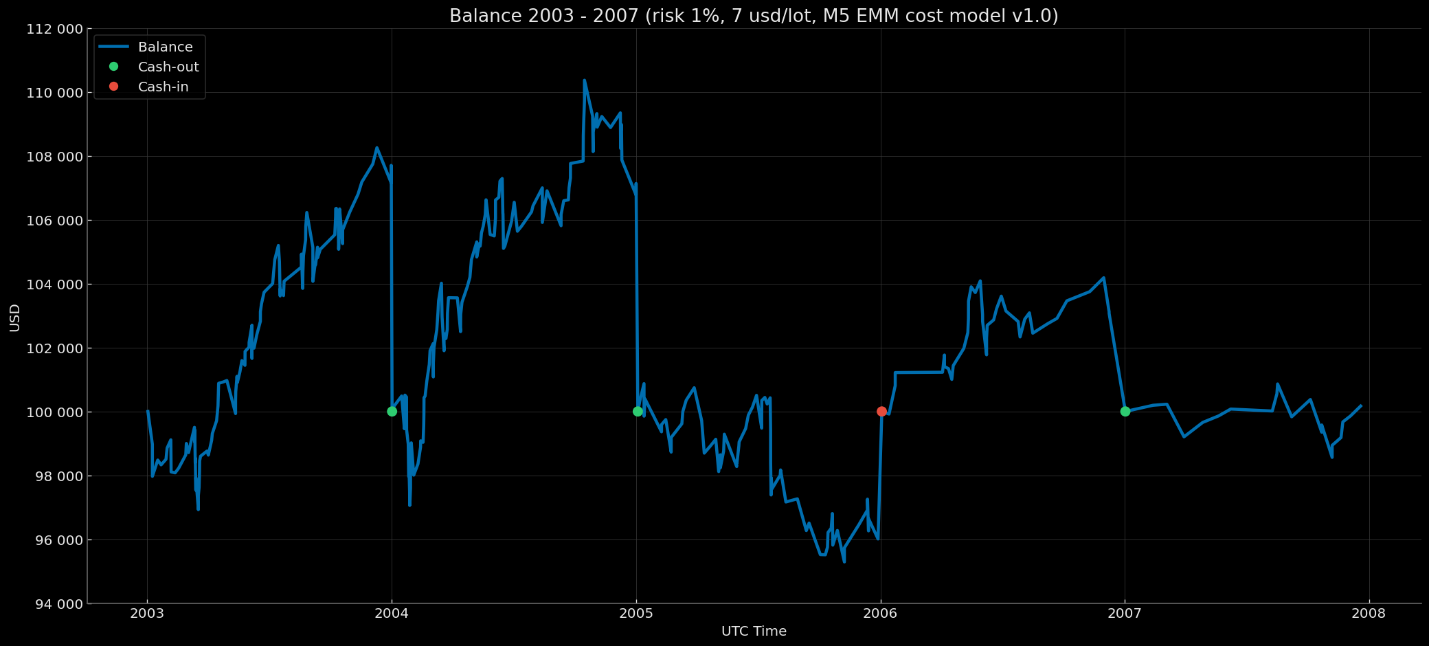
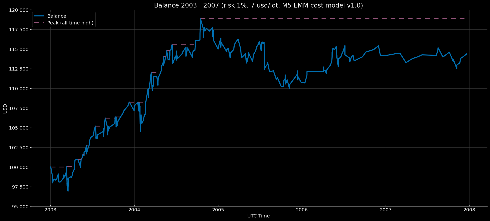
Retail Standard
Balance Curve — Fixed Start 100k & Compounding EoY-SoY Base 100k Modes (Risk 1%, $7 round-turn per standard lot, M5 EMM cost model v1.0) 2003–2007
|
|
Retail Rebate
Balance Curve — Fixed Start 100k & Compounding EoY-SoY Base 100k Modes (Risk 1%, $5 round-turn per standard lot, M5 EMM cost model v1.0) 2003–2007

|
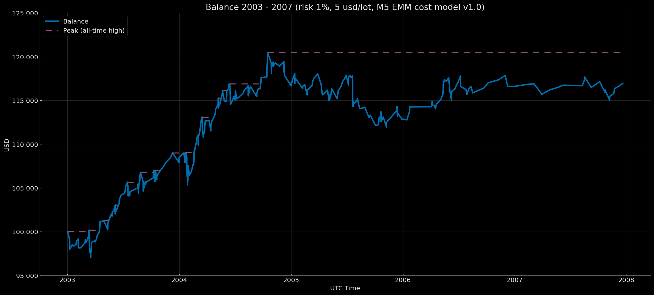
|
Balance Curve — Fixed Start 100k Mode (Risk 1%, $7 round-turn per standard lot, M5 EMM cost model v1.0) 2008–2025-08
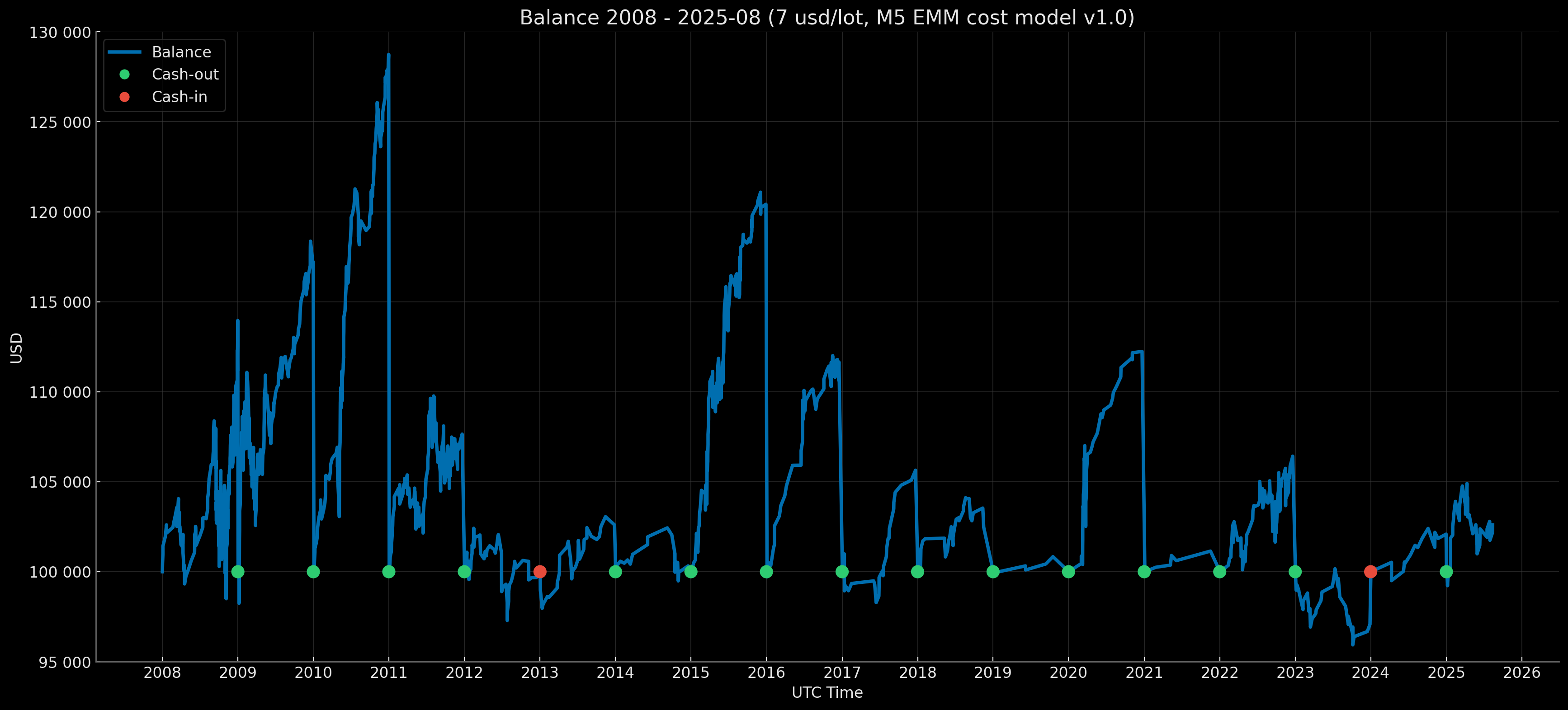
Balance Curve — Compounding EoY-SoY Base 100k Mode (Risk 1%, $7 round-turn per standard lot, M5 EMM cost model v1.0) 2008–2025-08
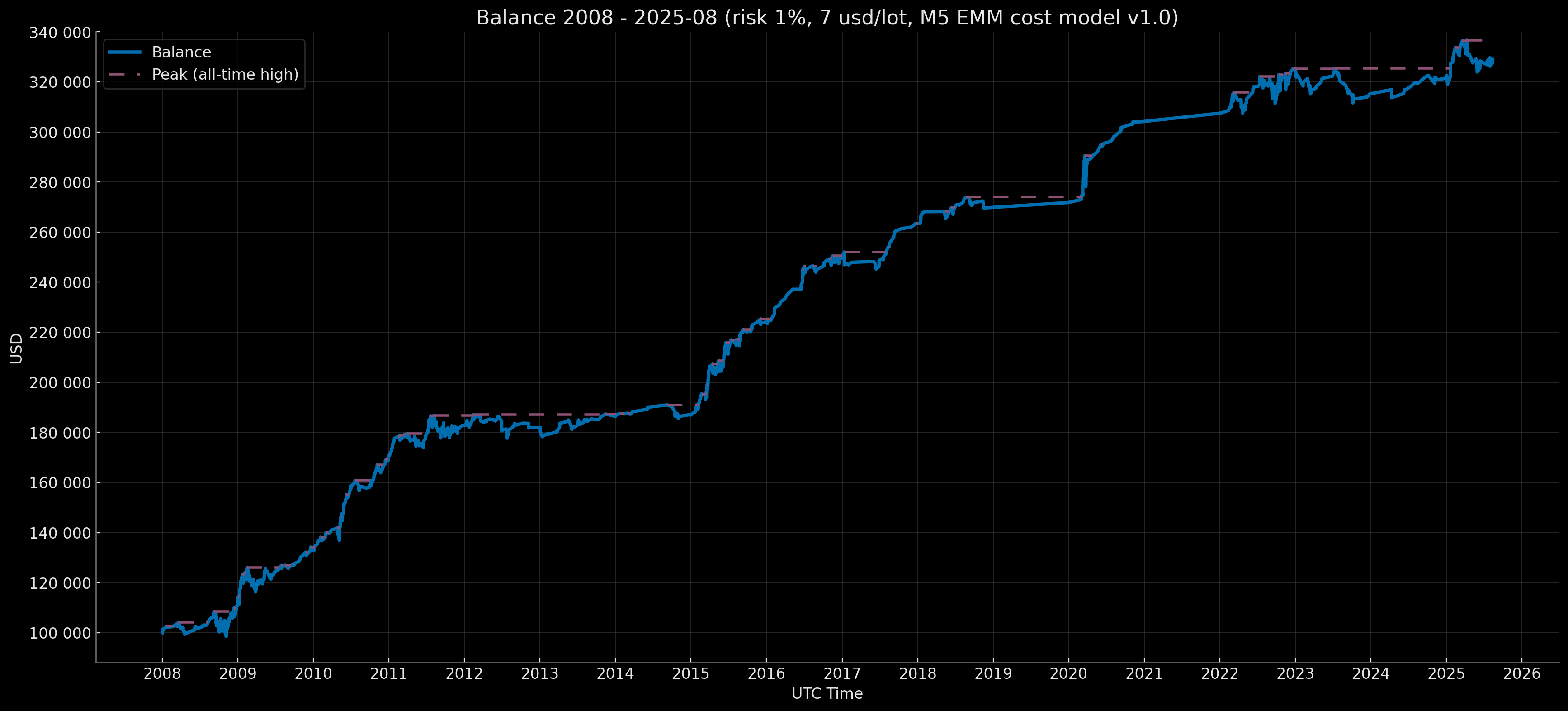
Retail Rebate
Balance Curve — Fixed Start 100k Mode (Risk 1%, $5 round-turn per standard lot, M5 EMM cost model v1.0) 2008–2025-08
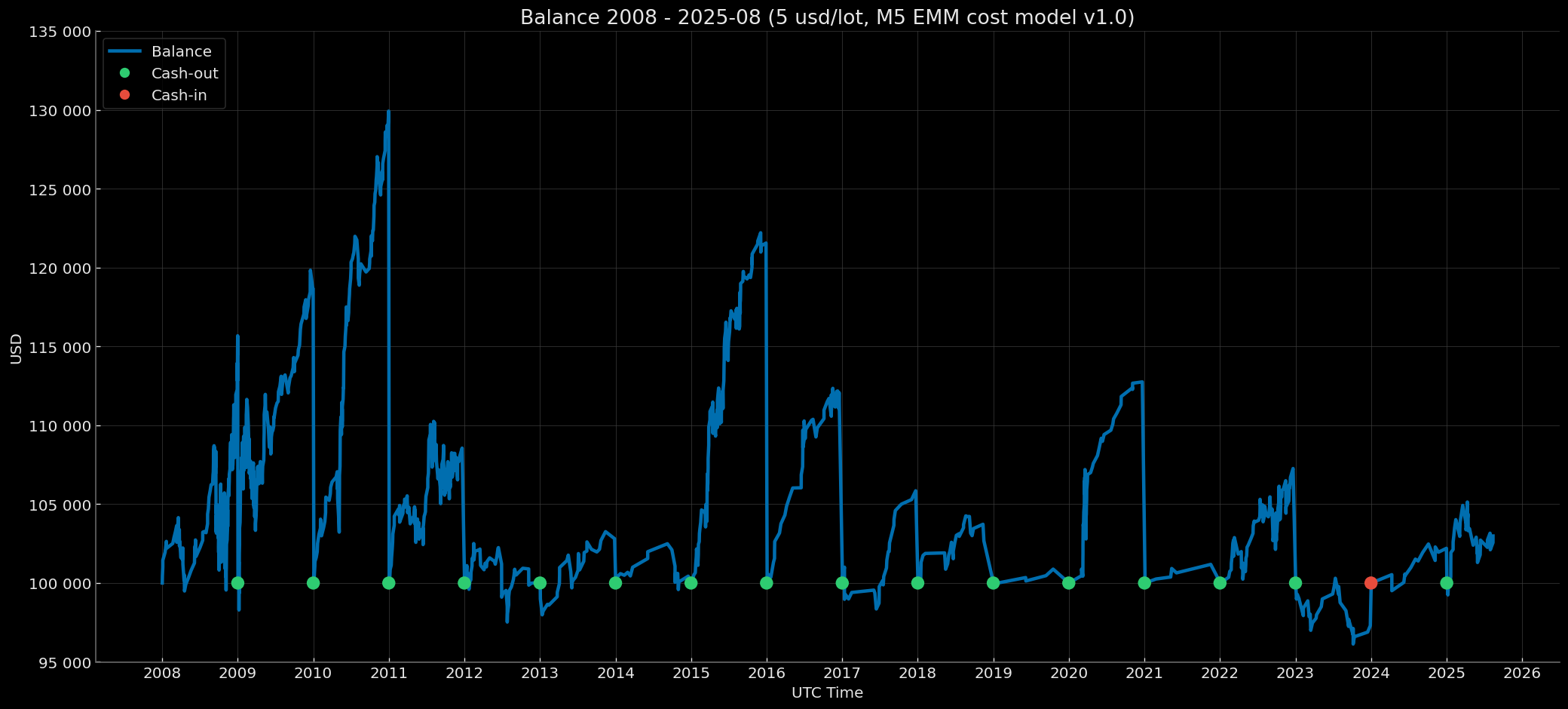
Balance Curve — Compounding EoY-SoY Base 100k Mode (Risk 1%, $5 round-turn per standard lot, M5 EMM cost model v1.0) 2008–2025-08
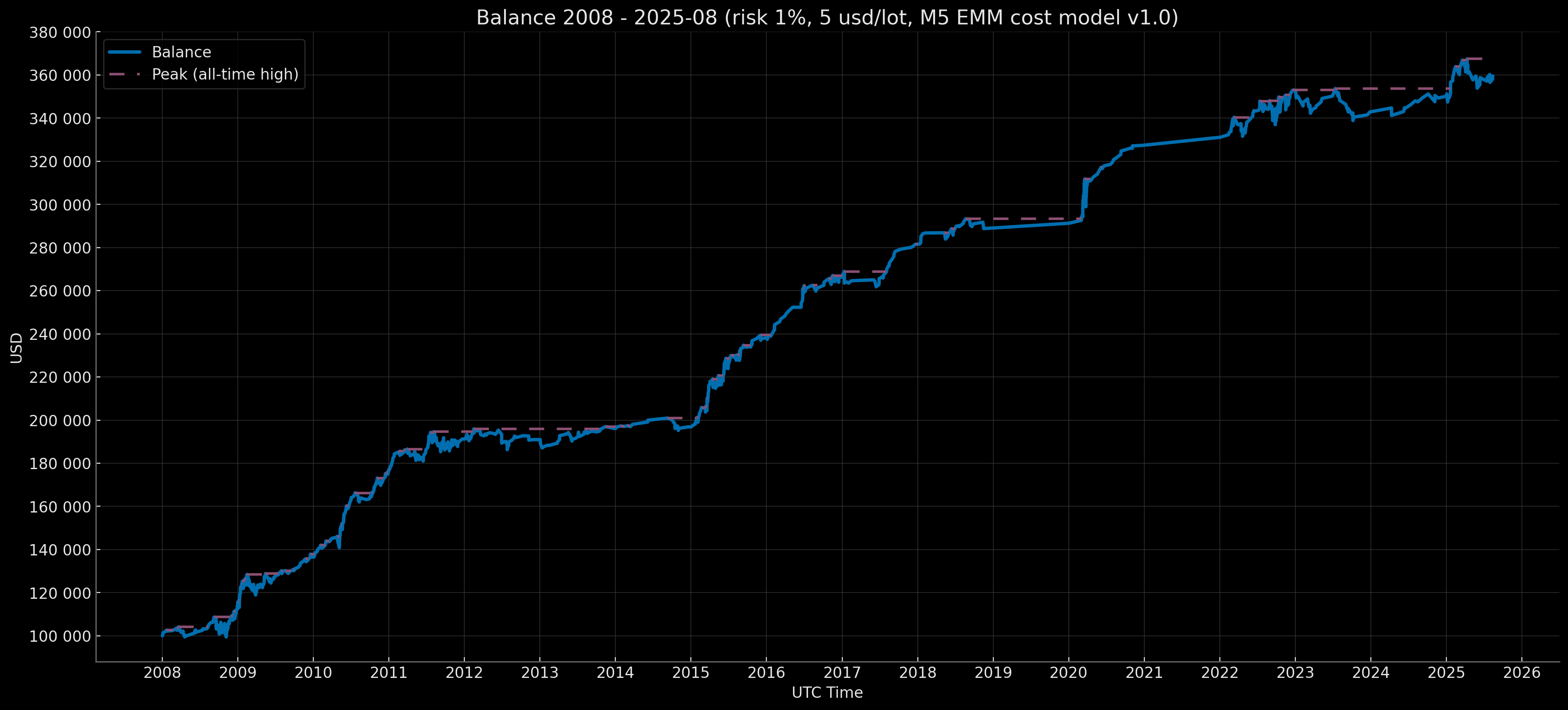
Institutional
Balance Curve — Notional 1M-5M Mode (Risk 1%, $5.5 round-turn per standard lot, M5 EMM cost model v1.0) 2008–2025-08
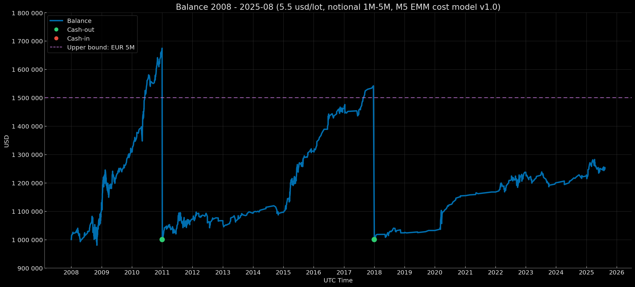
Balance Curve — Notional 5M-15M Mode (Risk 1%, $5.5 round-turn per standard lot, M5 EMM cost model v1.0) 2008–2025-08
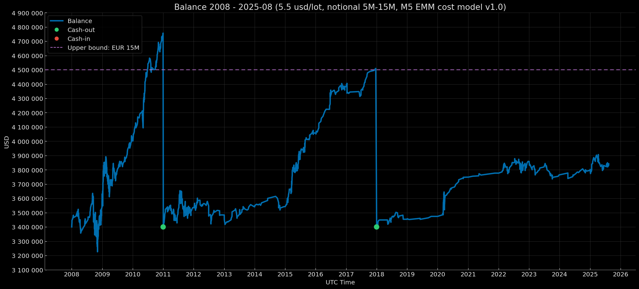
Balance Curve — Notional 15M-30M Mode (Risk 1%, $5.5 round-turn per standard lot, M5 EMM cost model v1.0) 2008–2025-08
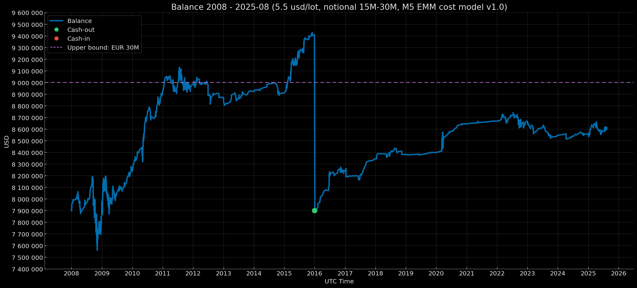
Balance Curve — Compounding EoY-SoY Base 100k Mode (Risk 1.5%, $5 round-turn per standard lot, M5 EMM cost model v1.0) 2003–2025-08
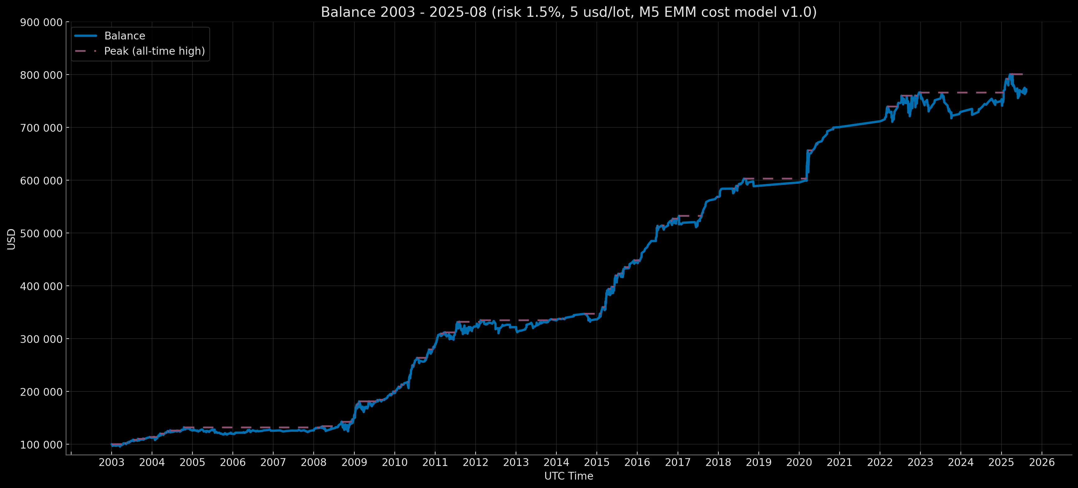
Robustness of Results
Robustness is demonstrated through performance profiles and capitalization regimes based on a dynamic cost model over a long historical horizon, as well as through a GBPUSD cross-asset test conducted before and after Brexit (2016).
Extended Baseline & Core Baseline
Retail Standard:
- Fixed Start 100k:
0.70 (commission) + 0.30 (spread) + 0.10 (slippage) = 1.10 pipsper trade - Compounding EoY–SoY Base 100k:
0.70 (commission) + dynamic (spread + slippage) as balance changes = 1.10–1.25 pipsper trade
Retail Rebate:
- Fixed Start 100k:
0.50 (commission) + 0.30 (spread) + 0.10 (slippage) = 0.90 pipsper trade - Compounding EoY–SoY Base 100k:
0.50 (commission) + dynamic (spread + slippage) as balance changes = 0.90–1.05 pipsper trade
Composite Baseline
Retail Rebate:
- Compounding EoY–SoY Base 100k:
0.50 (commission) + dynamic (spread + slippage) as balance changes = 0.90–1.40 pipsper trade
As a detailed robustness example, Institutional profiles fix costs by notional volume bands; when the end-of-year threshold is reached, the base balance is reset:
- Notional 1M–5M:
0.55 (commission) + 0.30 (spread) + 0.35 (slippage) = 1.20 pipsper trade - Notional 5M–15M:
0.55 (commission) + 0.50 (spread) + 0.85 (slippage) = 1.90 pipsper trade - Notional 15M–30M:
0.55 (commission) + 0.55 (spread) + 1.65 (slippage) = 2.75 pipsper trade
Summary: Across all profiles, modes, and Baseline tracks, the equity path remains sustainably positive with no catastrophic drawdowns; the effect persists under all modeled cost levels, as confirmed by the closed-equity curves.
GBPUSD Cross Asset Test
GBPUSD Cross Asset Test – Balance Curve — Compounding EoY-SoY Base 100k Mode (Risk 1%, no cost model) 2008–2025-08
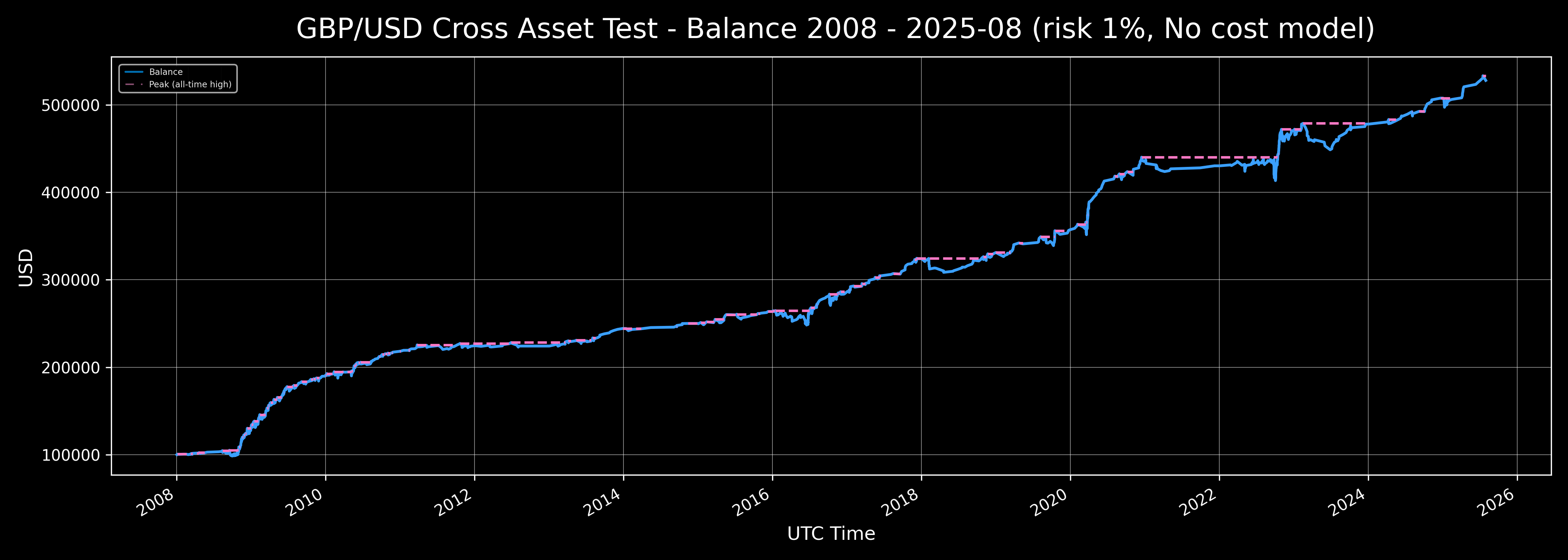
To demonstrate model robustness and the absence of overfitting, a cross-asset test was performed: parameters optimized on EURUSD were applied to GBPUSD without any adjustments for UK-specific economic data or volatility patterns.
Historically, EURUSD and GBPUSD were highly correlated, but after Brexit (2016) this correlation dropped significantly. This makes GBPUSD an independent out-of-sample test: the asset was not involved in optimization and has a materially different post-Brexit market structure.
Stable performance on GBPUSD confirms:
- absence of overfitting,
- no multiple testing or selection bias,
- the model’s ability to generalize without cherry-picking.
Even on degraded data (Stress period), the strategy did not exhibit catastrophic capital loss: the maximum balance decline in 2001 was ≈15%.
Full per-track reviews and source CSVs are available in the corresponding tracks.
- Overview: results/README.md
- Results: results/
Conclusions
Summarizing the material across all sections, the backtest results provide robust empirical evidence of invariant quantitative factors (signs of market inefficiency) in EUR/USD price dynamics, and they validate the correctness of the approach taken (transparency, reproducibility, absence of artificial “execution enhancements”) under the stated assumptions and a conservative execution model.
Additionally, the body of evidence presented in the methodology objectively supports a detailed and conservative approach to backtesting the core subset of the author’s model without attempts to overstate results:
- a thoroughly engineered engine with an emphasis on objective treatment of all relevant factors while operating under non-institutional infrastructure and resource constraints;
- granular cost modeling based on average trade sizes, risk parameters, and stop distances, aligned with the strategy’s trading windows;
- high transparency of inputs and reproducibility of the entire pipeline;
- a formalized Conditional Sortino (strict, loss-only) methodology: the metric is deliberately conservative (typically lower than standard Sortino) yet more relevant and objective, as it is oriented toward precise assessment of trading-strategy risk.
The invariance of the logic, the absence of re-training/“cherry-picking”/multiple testing and selection bias, and the objectivity of the results are further supported by:
- a cryptographically fixed version of the backtest engine and single-take live backtest videos with full verification of the engine version, input files, cost-model values, and obtained results;
- transparent metric computation based on non-public trade files and balance series (cryptographically fixed in the consolidated manifests generated by the backtest engine), including an open calculator script and a formalized methodology;
- a backtest over virtually the entire available historical horizon of the euro (since the introduction of cash in January 2002), which—together with a fixed engine version, live-run recordings, and illustrating dynamics via balance curves (built from
balance_YYYY.csv)—effectively rules out the influence of multiple testing and selection bias, as well as the risk of segment-specific “fit”; this is additionally corroborated by 12/36-month rolling evaluations, drawdown quantiles, Trade bootstrap (EDR and sequences of losing trades), detailed Monte Carlo (stationary bootstrap), and BCa confidence intervals at a 90% confidence level. - GBPUSD cross-asset test results for the period 2008–2025-08 using unchanged parameters.
Limitations and scope of applicability
- The results pertain to currency pairs (EUR/USD & GBP/USD) and a single signal timeframe (M5).
- Execution is modeled on M1 with a conservative cost model; tick-level execution is not modeled.
- The canonical specification for M1 data is the raw HistData series. For the backtest, only the timestamp conversion from fixed EST to UTC was performed.
- Historical data quality is non-uniform (see Data Quality Policy v1.0).
- Stress periods (2001–2002) are excluded from the aggregate metrics; for them, only yearly backtest tallies are published.
- This backtest is a deterministic demonstration using M1 data, a conservative cost model, and strict liquidity/news/gap filters. It does not purport to resolve microstructure questions (tick sequencing/queueing, limit order book, latency, market impact); such issues are addressed exclusively in institutional settings. The conservative assumptions are intentional: the objective is to understate, not embellish, the results.
Links
- Euro MacroMechanica (EMM) Backtesting Ecosystem
- Full verification guide to process transparency and the input/output files used in the backtest
- Guide to verifying SHA-256, GPG signatures, and OTS
- Backtest results
- metrics-toolkit
- data-hub
- data-preparation-toolkit
Contact
GitHub: rleydev (thelaziestcat) · Email: thelazyazzcat@gmail.com, thelazziestcat@proton.me
Licenses & Attributions
- Repository license map (results) – LICENSES.md
- Code and utilities in related repositories are governed by their respective licenses; see each repository’s
LICENSE. - The strategy source code, detailed trade reports, and balance series (with timestamps and prices) are non-public.
Disclaimer — Not Investment Advice
This material is provided for informational and research purposes only and does not constitute investment advice, an offer, or a solicitation. Backtested results are hypothetical and subject to limitations; past performance is not indicative of future results. Assumptions (cost models, risk, etc.) are illustrative and may not align with the reader’s objectives or constraints.